Subject Line
2 way lookup is amazing
Overview
Sometimes you may want to lookup a value in a table using both rows and columns. You can build your own formula that to perform a two-way lookup with help of INDEX and MATCH function.
Syntax
=INDEX(data,MATCH(val,rows,0),MATCH(val,columns,0))
Let’s understand both the function
INDEX function returns a value in a table based on the intersection of a row and column position within that table.
Syntax
=INDEX (array, row_num, [col_num], [area_num])
Arguments
· array – A range of cells, or an array constant.
· row_num – The row position in the reference or array.
· col_num – [optional] The column position in the reference or array.
· area_num – [optional] The range in reference that should be used.
Match option is used to locate the position of a lookup value in a row, column, or table.
=MATCH (lookup_value, lookup_array, [match_type])
Arguments
· lookup_value – The value to match in lookup_array.
· lookup_array – A range of cells or an array reference.
· match_type – [optional] 1 = exact or next smallest (default), 0 = exact match, -1 = exact or next largest.
Working
Let’s understand the working with the help of an example.
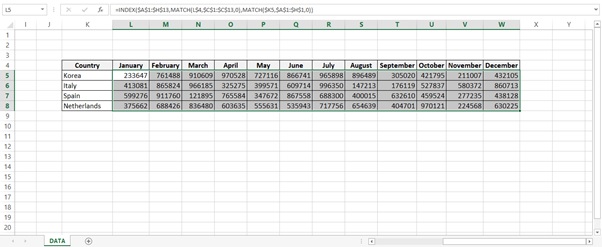
We have a report (Figure 1: Sales Report) for the year 2018.
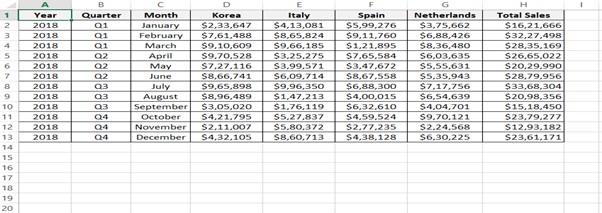
Figure 1: Sales Report
The management wants to find the sales amount from the sales table using a different format.
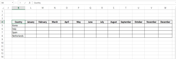
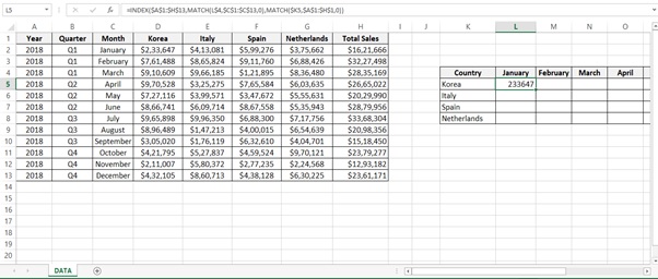
Step 1: Let’s find out the Sales of Korea for January month.
Type the below formula
=INDEX($A$1:$H$13,MATCH(L$4,$C$1:$C$13,0),MATCH($K5,$A$1:$H$1,0))
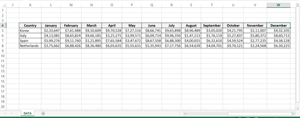
Step 2: Drag the formula for all the countries.
Select the cells and press Ctrl+D
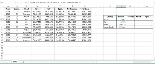
Step 3: Drag the formula to all the months
Select the cells and do Ctrl+R
Step 4: Final result after formatting the currency.
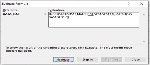
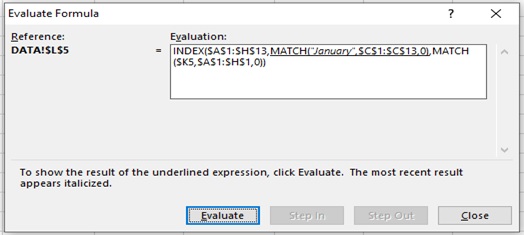
Understanding how the formula works with the help of Evaluate Formula
Step 1: Select the cell (L5 in this case) that you want to evaluate. Only one cell can be evaluated at a time.
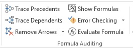
Step 2: On the Formulas tab click on Evaluate Formula in Formula Auditing group
Step 3: Evaluate Formula dialog box will appear.
Step 4: Click Evaluate to examine the value of the underlined reference. The result of the evaluation is shown in italics.
If the underlined part of the formula is a reference to another formula, click Step In to display the other formula in the Evaluation box. Click Step Out to go back to the previous cell and formula.
Step 5: January is the result and checks the Row no.
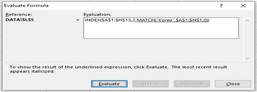
Step 6: Check the Column $K5

Step 7: Korea is the result
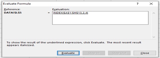
Step 8: Returns the column no. 4
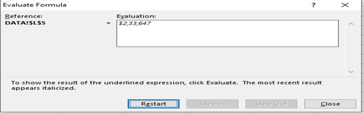
Step 9: Result
Scope of usage
ü Can be used to perform a two way lookup
ü Can be used with the INDEX () function and MATCH () function
ü Can be much faster than VLOOKUP
ü Can be used to return a reference rather than a value, which allows us to use it for more purposes