Subject Line
The magic of GETPIVOTDATA () will protect your values ….
Overview
Sometimes the management may request for different set of reports summarized based on different conditions. You need not create a pivot table every time. With the help of GETPIVOTDATA we can extract correct data from the Pivot table even if the pivot table layout is changed as it uses criteria to lookup.
Generate GetPivotData feature
To enter the formula you can type equal to (=) and click on the specified cell in the pivot table. If you give reference to a cell by typing the cell i.e. $D$9 then the value will change if the layout is changed as it refers to that particular cell only.
If you have the Generate GetPivotData feature turned on, this formula will be created automatically, when you reference a cell in a Pivot Table.
If you prefer to use a cell reference, you can type the reference, e.g. = B5
OR, use the Generate GetPivotData command to turn this feature off.
How to toggle (turn on/turn off) the GetPivotData feature
- Select any cell in a pivot table.
- On the Ribbon, under PivotTable Tools, click the Options tab
- In the PivotTable group, click the drop down arrow for Options
- Click the Generate GetPivotData command, to turn the feature off or on.
Syntax
Let’s understand the syntax of GETPIVOTDATA () function
GETPIVOTDATA (data_field, pivot_table, [field1, item1, field2, item2], …)
The GETPIVOTDATA function syntax has the following arguments:
- Data_field -The Field in the Values area of the Pivot Table
- Pivot table- The pivot table you are selecting i.e. Can choose anywhere in the Pivot Table but we usually select the cell in the top left hand corner
- Field -Field name from your Pivot Table
- Item- Item from within your Field i.e. This can be referenced to a cell outside the Pivot Table
Working
Let’s understand the working with the help of an example below. (Figure 1: Sales of Laptops across Countries)
We have a table with Sales of Laptop for the year 2017 & 2018 (Quarter wise) for Korea, Italy, Spain and Netherlands. The Sales figures are in USD
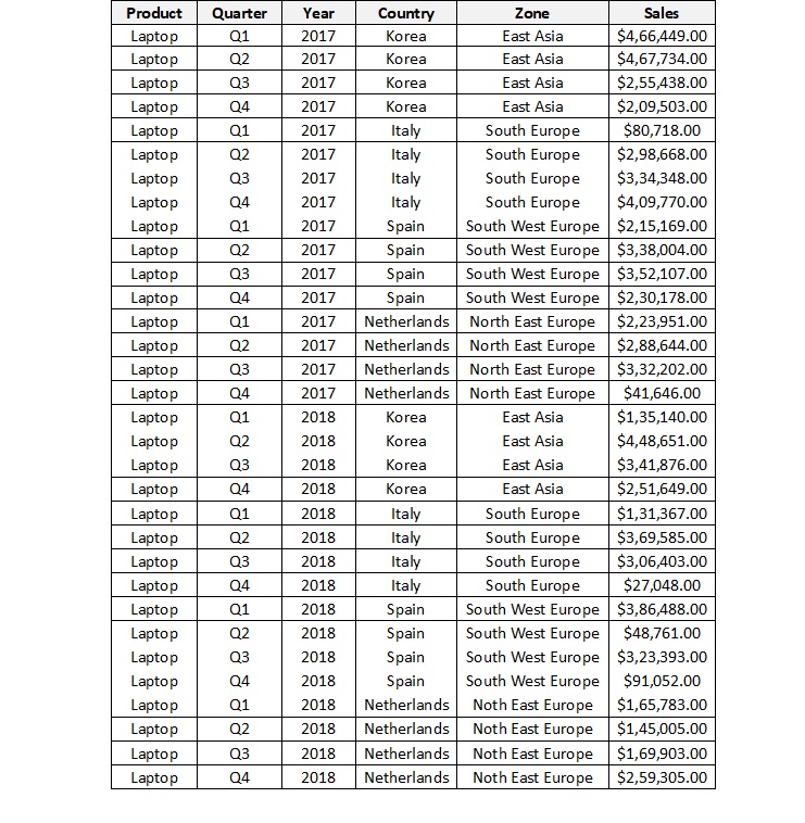
Figure 1: Sales of Laptops across Countries
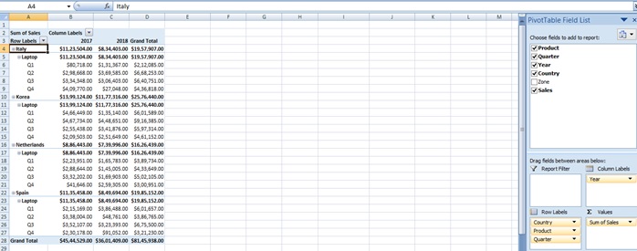
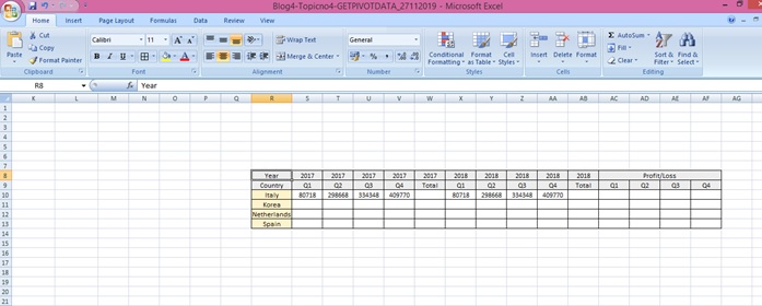
Step 1: Create a pivot table as shown in the below image.
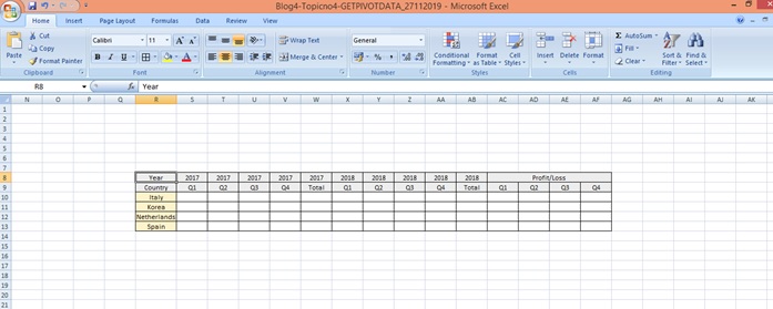
Step 2: Our goal here is to fill the table for the year 2017 & 2018 and find the out the Profit and Loss country wise report which has been asked by the management
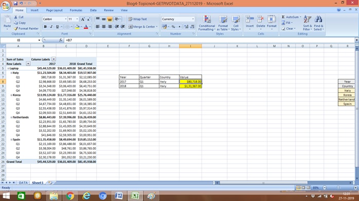
Step 3: Select cell S10 and type = and click on cell B6.
You will get the formula as shown in the below screenshot
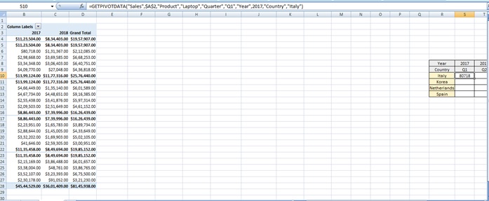
Step 4: Customize the formula (to fix the quarter)
=GETPIVOTDATA (“Sales”,$A$2,”Product”,”Laptop”,”Quarter”,S$9,”Year”,$S$8,”Country”,$R$10)
Drag to the right hand side till year 2017
Step 5: Repeat this for year 2018 and fill the table (for each country and each year)
Total of 2017 will Total of Q1+Q2+Q3+Q4 for 2017 and for 2018 will be Total of Q1+Q2+Q3+Q4 for 2018
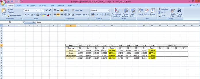
Step 6: Calculate the Profit and Loss (each Qtr 2018 minus corresponding Qtr 2017 values)
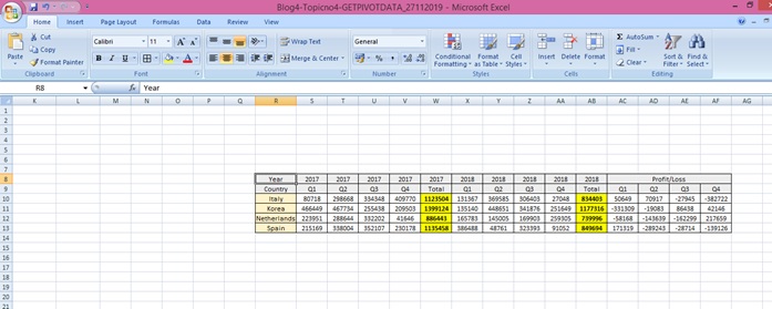
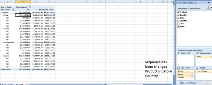
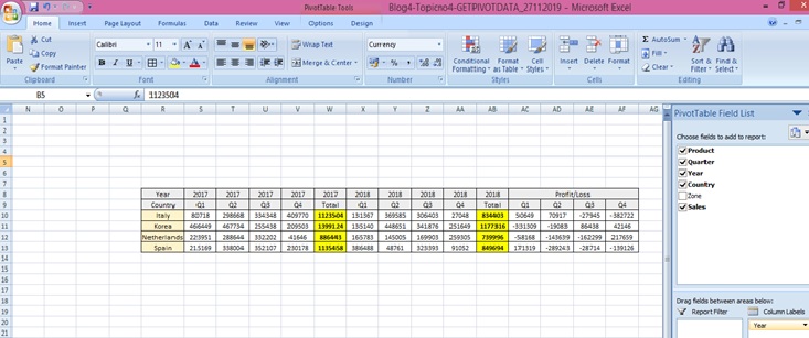
Step 7: Let’s change the table layout of the Pivot table. Drag the Product before the Country as asked by the management.
Step 8: Result is the same and there is no change to the report
Step 9: Let’s filter the year 2018 and see the difference.
A #REF error (the “ref” stands for reference) is the message Excel displays when a formula references a cell that no longer exists, usually caused by deleting cells that a formula is referring to.
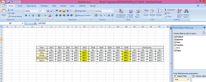
Step 10: After the year is added to the pivot table the values get restored
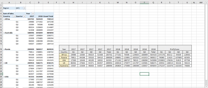
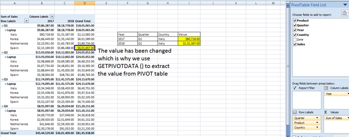
Step 11: We are understanding the difference between reference and GETPIVOTDATA () by creating a new table and referencing the values first
Now if you change the sequence of the Row labels i.e. you drag Quarter above product you get the result as below
Scope of Usage:
- Can be used to protect the value of the pivot table even if the reference changes
- Can be used to search the actual value based on search criteria in the GETPIVOTDATA ()
- Can be used to extract the value even if the report layout is changed
- Can be used to customize charts which is not possible by PivotChart option
- Can be used to automatically make changes if pivot table is refreshed