Subject Line
Use Exact () for case sensitive values
Overview
As you already know a usual VLOOKUP () formula is case sensitive and will ignore case. Sometimes you may want to lookup exact value in a table. Hence we use Exact () function along with INDEX & MATCH function with an array formula to retrieve the desired result from the table.
Working of Functions
Let’s understand what INDEX (), MATCH () & EXACT () function does.
INDEX function returns a value in a table based on the intersection of a row and column position within that table.
Syntax
=INDEX (array, row_num, [col_num], [area_num])
Arguments
· Array – A range of cells, or an array constant.
· row_num – The row position in the reference or array.
· col_num – [optional] The column position in the reference or array.
· area_num – [optional] The range in reference that should be used.
Match option is used to locate the position of a lookup value in a row, column, or table.
Syntax
=MATCH (lookup_value, lookup_array, [match_type])
Arguments
· lookup_value – The value to match in lookup_array.
· lookup_array – A range of cells or an array reference.
· match_type – [optional] 1 = exact or next smallest (default), 0 = exact match, -1 = exact or next largest.
Exact option is used to compare 2 text strings
Syntax
=Exact (Text1,Text2)
Arguments
· Text1 – First text string to compare
· Text2 – Second text string to compare
Working
Let’s understand the working with the help of an example.
We have a report (Figure 1: Sales Report) for the year 2018.
We want to find out Sales done by the respective Sales Rep.
Vlookup () function will search the first value which is not case sensitive and might not extract the desired result and does not consider case
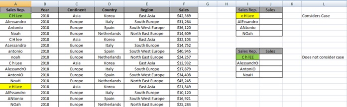
Figure 1: Sales Report
Step 1: Type the below formula in J2 Cell
=INDEX($F$2:$F$17,MATCH(TRUE,EXACT($I2,$A$2:$A$17),0))
What is Array Formula
An array formula is a formula that can perform multiple calculations on one or more items in an array.
Since this is an array formula, use it with Control + Shift + Enter, instead of just Enter.
{=INDEX($F$2:$F$17,MATCH(TRUE,EXACT($I2,$A$2:$A$17),0))}
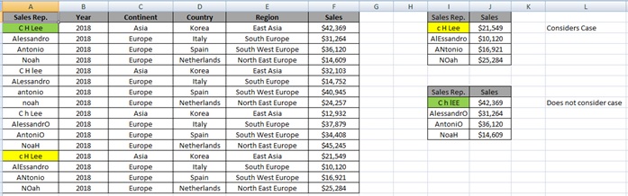
We get the desired result

Step 2: Select J2:J5 and Press Ctrl+D
Understanding how the formula works with the help of Evaluate Formula
Step 1: Select the cell (J2 in this case) that you want to evaluate. Only one cell can be evaluated at a time.
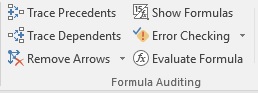
Step 2: On the Formulas tab click on Evaluate Formula in Formula Auditing group
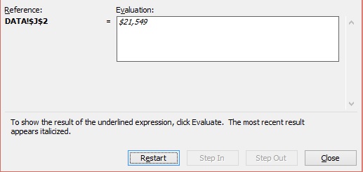
Step 3: Evaluate Formula dialog box will appear.
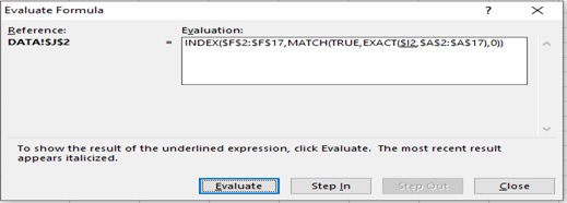
Step 4: Click Evaluate to examine the value of the underlined reference. The result of the evaluation is shown in italics.
If the underlined part of the formula is a reference to another formula, click Step In to display the other formula in the Evaluation box. Click Step Out to go back to the previous cell and formula.
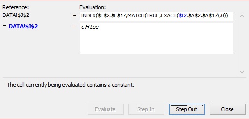
Step 5: Click on Evaluate
Exact function will be executed
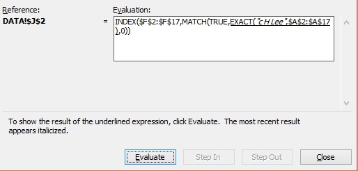
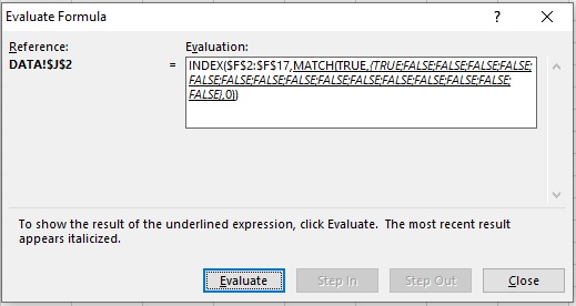
Step 6: Click on Evaluate
Exact function is being evaluated
Step 7: Click on Evaluate
Match function is executed
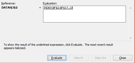
Step 8: Result
Scope of usage
ü Can be used to compare case
ü Can be used to perform a case sensitive lookup
ü Can be used instead of VLOOKUP () function
ü Can be used as an array formula
ü Can be used to retrieve both text and numeric values