Subject Line
You don’t need a helper for lookup all the time
Overview
Sometimes you may need to get the output without using helper column. What is a helper column? We create a separate column and concatenate both the values in a separate column and then use it as a lookup value to get the desired result. But in order to do this without a helper column, we will have to combine VLOOKUP function along with CHOOSE function to get the desired result.
Working
Lets understand the working of VLOOKUP () function
Syntax
VLOOKUP ( value, table, index_number, [approximate_match] )
Arguments
· The value you want to look up which is called the lookup value
· The range where the lookup value is located
Note: the lookup value should always be in the first column in the range for VLOOKUP to work correctly. For example, if your lookup value is in cell C2 then your range should start with C.
The column number in the range that contains the return value
For example, if you specify B2:D11 as the range, you should count B as the first column, C as the second, and so on.
Optionally, you can specify TRUE if you want an approximate match or FALSE if you want an exact match of the return value. If you don’t specify anything, the default value will always be TRUE or approximate match. You can also use 1 or 0
Lets understand the working of CHOOSE () function
Syntax
=CHOOSE (index_num, value1, [value2], …)
Arguments
· index_num – The value to choose. A number between 1 and 254.
· value1 – The first value from which to choose.
· value2 – [optional] The second value from which to choose.
Let’s understand with the help of an example.
Below is the table (Figure 1: Sales Report) which contains sales (amount in USD) done by Sales representative for the Year 2018. We need to find the Sales done by Sales Rep. for Q1, Q2, Q3, Q4.
Hint: We have to combine Sales Rep. and Quarter as Lookup Value to get the correct output.
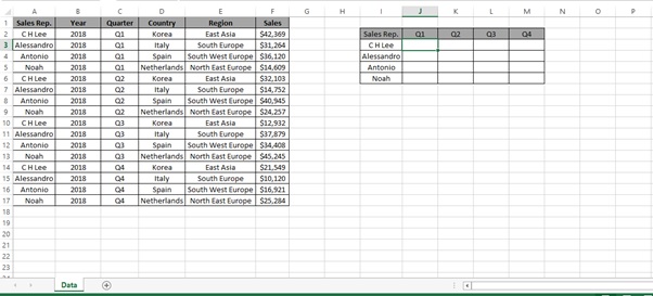
Figure 1: Sales Report
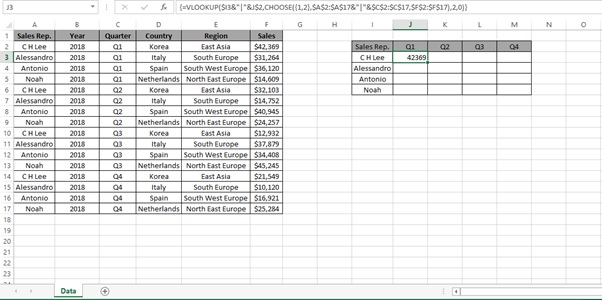
Step 1: Type the below formula
=VLOOKUP($I3&”|”&J$2,CHOOSE({1,2},$A$2:$A$17&”|”&$C$2:$C$17,$F$2:$F$17),2,0)
What is Array Formula:
An array formula is a formula that can perform multiple calculations on one or more items in an array.
Since this is an array formula, use it with Control + Shift + Enter, instead of just Enter.
{=VLOOKUP($I3&”|”&J$2,CHOOSE({1,2},$A$2:$A$17&”|”&$C$2:$C$17,$F$2:$F$17),2,0)}
We get the desired result
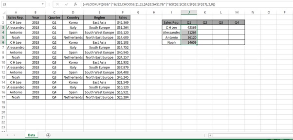
Step 2: Select the cells from J3 to J6 and press Ctrl + D
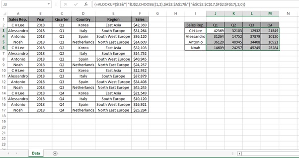
Step 3: Select the cells from J3 to J6 and Select till Column M and press Ctrl + R
Understanding how the formula works with the help of Evaluate Formula
Step 1: Select the cell (J3 in this case) that you want to evaluate. Only one cell can be evaluated at a time.
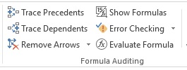
Step 2: On the Formulas tab click on Evaluate Formula in Formula Auditing group
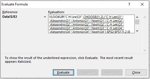
Step 3: Evaluate Formula dialog box will appear.
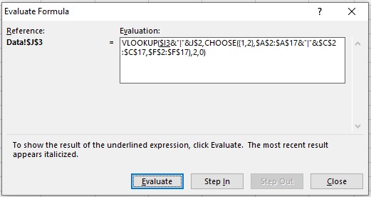
Step 4: Click Evaluate to examine the value of the underlined reference. The result of the evaluation is shown in italics.
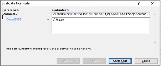
If the underlined part of the formula is a reference to another formula, click Step In to display the other formula in the Evaluation box. Click Step Out to go back to the previous cell and formula.
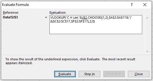
Step 5: Click on Evaluate
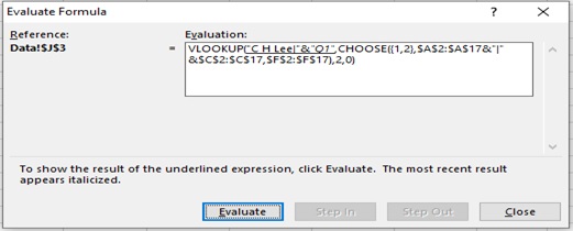
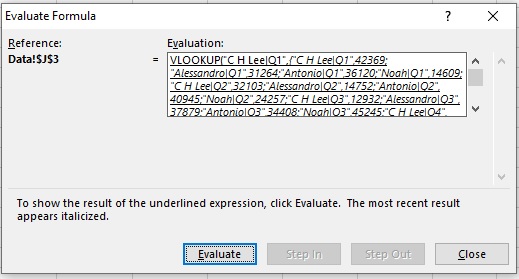
Step 6: Click on Evaluate
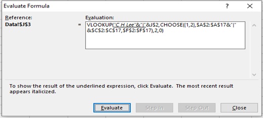
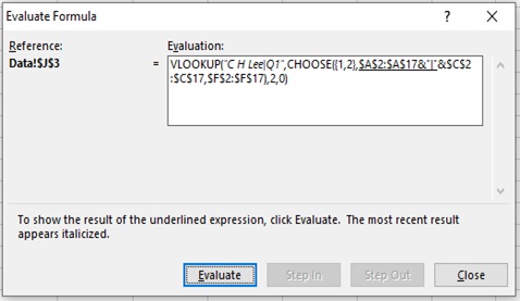
Step 7: Click on Evaluate
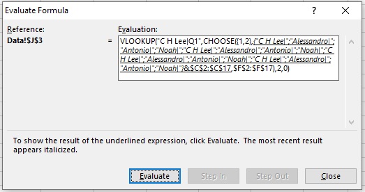
Step 8: Click on Evaluate
Step 9: Click on Evaluate
Step 10: Click on Evaluate
Step 11: Click on Evaluate
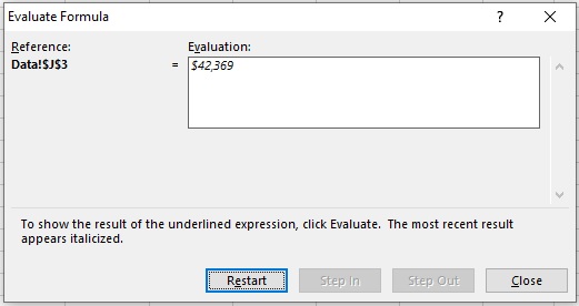
Step 12: Result
Scope of usage
ü Can be used without the need for a separate helper column
ü Can be used to lookup multiple criteria by using VLOOKUP () & CHOOSE () Function