Overview
Sometimes you may need to look up the 2nd,3rd,4th or Nth value from a table i.e. based on the occurrences of the values dynamically lookup for the values. VLOOKUP () Function lookups a value from left side of the column and returns the first matching value based on column index number. We have to use the below formulas to get the desired result
Syntax
=INDEX(data,MATCH(val,rows,0),MATCH(val,columns,0))
INDEX function returns a value in a table based on the intersection of a row and column position within that table.
Syntax
=INDEX (array, row_num, [col_num], [area_num])
Arguments
· array – A range of cells, or an array constant.
· row_num – The row position in the reference or array.
· col_num – [optional] The column position in the reference or array.
· area_num – [optional] The range in reference that should be used.
Syntax
=SMALL(array, k)
Arguments
· Array – An array or range of numerical data for which you want to determine the k-th smallest value.
· K -The position (from the smallest) in the array or range of data to return.
Syntax
=IF (logical_test, [value_if_true], [value_if_false])
Arguments
· logical_test – A value or logical expression that can be evaluated as TRUE or FALSE.
· value_if_true – [optional] The value to return when logical_test evaluates to TRUE.
· value_if_false – [optional] The value to return when logical_test evaluates to FALSE.
Syntax
=ROW ([reference])
Arguments
· reference – [optional] A reference to a cell or range of cells.
Syntax
=COLUMNS (array)
Arguments
o array – A reference to a range of cells.
Syntax
=IFERROR (value, value_if_error)
Arguments
· value – The value, reference, or formula to check for an error.
· value_if_error – The value to return if an error is found.
Working
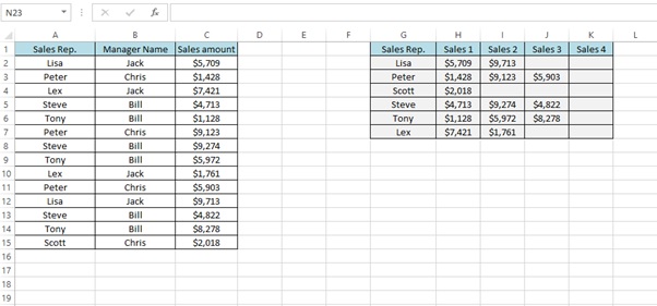
Let’s understand with the help of an example. Below is the table (Figure 1: Sales Report) which contains sales (amount in USD) generated by Sales representative along with their manager’s name.
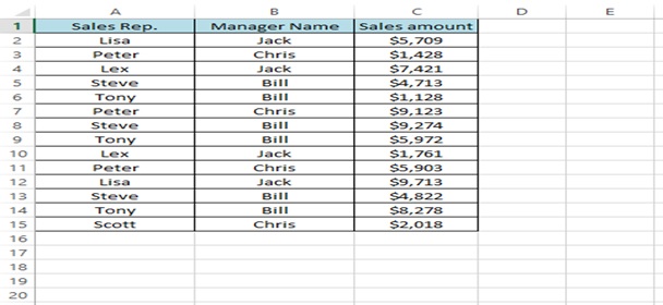
Figure 1: Sales Report
The management wants a report to show each Sales amount done by each sales person
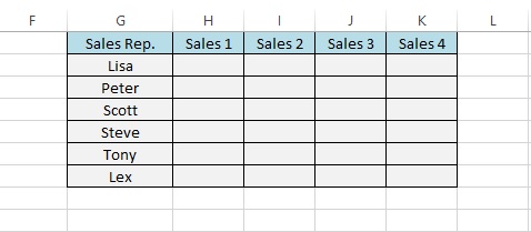
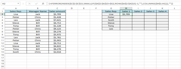
Step 1: Type the formula to get the desired result.
=IFERROR(INDEX($C$2:$C$15,SMALL(IF($A$2:$A$15=$G2,ROW($A$2:$A$15)-1,””),COLUMNS($H$1:H1))),””)
Copy this formula and paste it in cell H2.
What is Array Formula:
An array formula is a formula that can perform multiple calculations on one or more items in an array.
Since this is an array formula, use it with Control + Shift + Enter, instead of just Enter.
{=IFERROR(INDEX($C$2:$C$15,SMALL(IF($A$2:$A$15=$G2,ROW($A$2:$A$15)-1,””),COLUMNS($H$1:H1))),””)}
We get the desired result
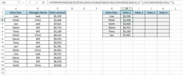
Step 2: Drag the Formula from H2 to H7
Step 3: Drag the formula from H2 to H7 to K Column (To the right)
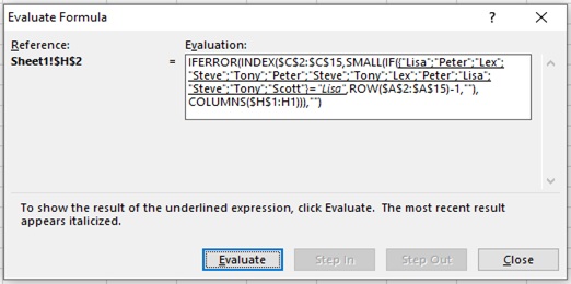
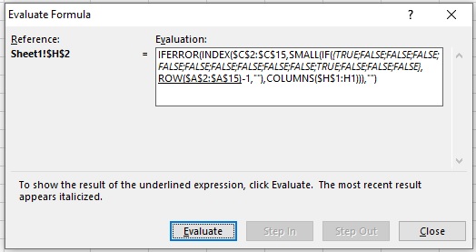
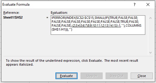
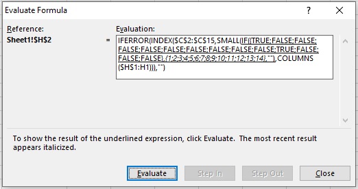
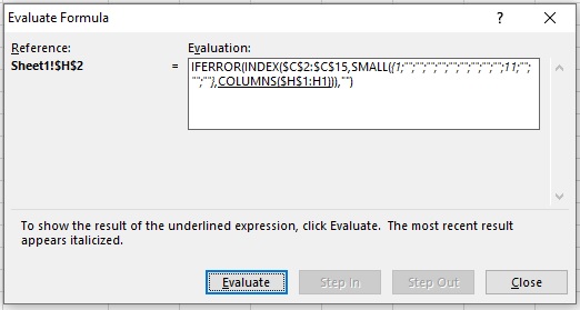
Understanding how the formula works with the help of Evaluate Formula
Step 1: Select the cell (H2 in this case) that you want to evaluate. Only one cell can be evaluated at a time.
Step 2: On the Formulas tab click on Evaluate Formula in Formula Auditing group
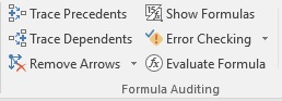
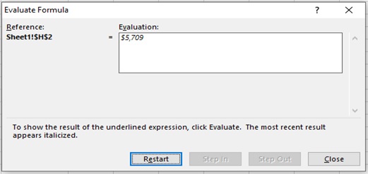
Step 3: Evaluate Formula dialog box will appear.
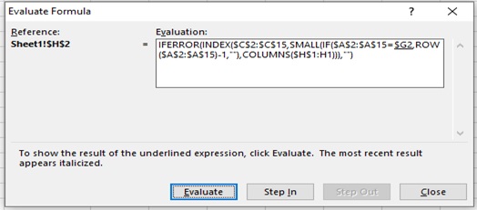
Step 4: Click Evaluate to examine the value of the underlined reference. The result of the evaluation is shown in italics.
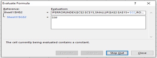
If the underlined part of the formula is a reference to another formula, click Step In to display the other formula in the Evaluation box. Click Step Out to go back to the previous cell and formula.
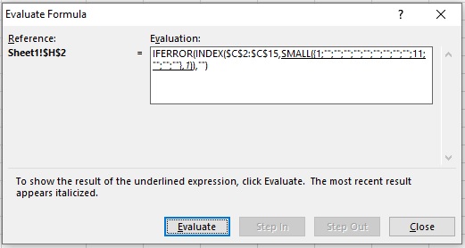
Step 5: Click on Evaluate
Step 6: Click on Evaluate
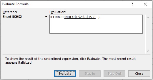
Step 7: Click on Evaluate
Step 8: Click on Evaluate
Step 9: Click on Evaluate
Step 10: Click on Evaluate
Step 11: Click on Evaluate
Step 12: Click on Evaluate
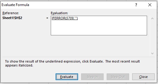
Step 13: Result
Scope of usage
ü Can be used as a dynamic lookup for values
Can be used to extract the nth occurrence