Overview

Sometimes you may want to make specific data stand out in your spreadsheet and capture the viewer’s attention. You can do that using conditional formatting. Conditional formatting helps you identify important cells in a table based on the conditions you specify.

Conditional formatting includes the below options:

• Highlight cell rules
• Top and bottom rules
• Data bars
• Color scales
• Icon sets

Working

Let’s understand the working with an example.

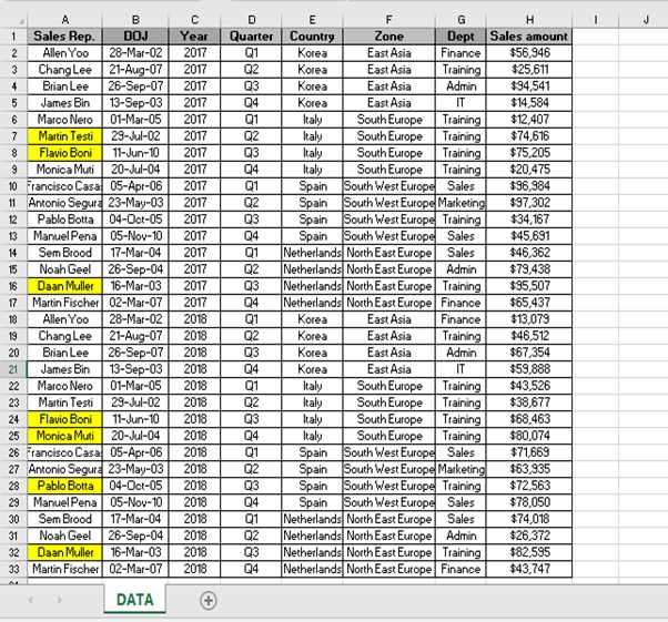
We have (Figure 1: Sales Report) for 4 countries for the Year 2017 & 2018.

We want to find out the Sales Rep name who works for “Training” Department and whose salary is greater than 50000$ using conditional formatting.

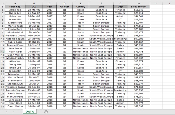
Figure 1: Sales Report

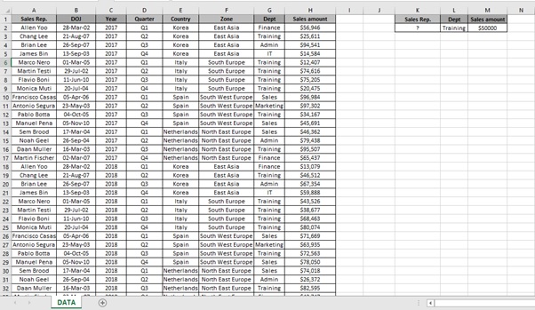
Step 1: Select the Sales Rep range (A2:A33) as we want to highlight the Sales Rep name only.

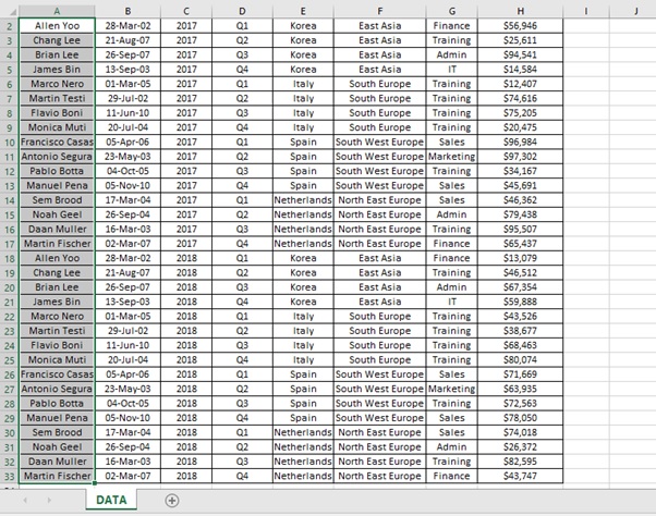
Step 2: Go to HOME tab

Step 3: Click on Conditional Formatting option in the Styles group.

Step 4: Click on New Rule.

Step 5: New Formatting Rule dialog box appears

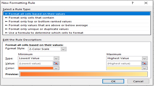
Step 6: Select “Use a formula to determine which cells to format” from the Select a Rule Type as we are going to use formula to highlight the cells.

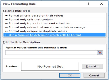
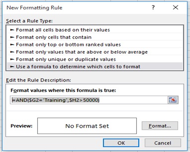
Step 7: Type the below formula in the formula bar

=AND($G2=”Training”,$H2>50000)

Step 8: Click on Format

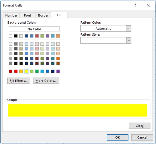
Step 9: Select the formatting.

I will use Yellow Color to format the cells from Fill option.

Step 10: Click on OK

 

Step 11: Click on OK

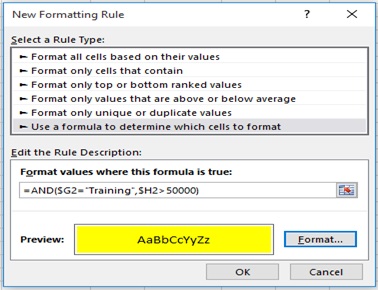
Step 12: Sales Rep. is highlighted as per condition provided.

You can also check, Add, Edit and Delete the conditional formatting rule through conditional formatting rules manager.

Steps are as follows.

Step 1: Go to HOME tab

Step 2: Click on Conditional Formatting option in the Styles group.

Step 3: Click on Manage Rules

Step 4: New Formatting Rule dialog box appears

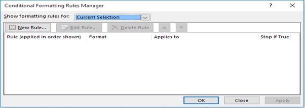
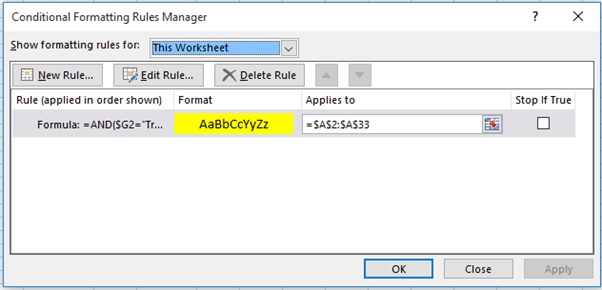
Step 5: Select This Worksheet Option from the Show formatting Rules Manager drop down.

Step 6: In the below image you can see the Rule(Formula),Format(Color),Applies to(Sales Rep. range) which was created earlier.

Scope of Usage

• Can be used to highlight important information
• Can be used for visual representation
• Can be used to get a quick idea of hidden patterns