Subject Line
Customizing the (hash) #N/A error
Overview
Sometimes when you don’t find the lookup value using VLOOKUP () function you will get the (hash) #N/A error. #N/A means “not available” or “no value available”). You may want to replace the #N/A message with a customised value then VLOOKUP () function should be nested inside the IFERROR () function.
Let’s also understand the working of VLOOKUP () function
- The value you want to look up which is called the lookup value
- The range where the lookup value is located
Note: the lookup value should always be in the first column in the range for VLOOKUP to work correctly. For example, if your lookup value is in cell C2 then your range should start with C.
- The column number in the range that contains the return value. For example, if you specify B2:D11 as the range, you should count B as the first column, C as the second, and so on.
- Optionally, you can specify TRUE if you want an approximate match or FALSE if you want an exact match of the return value. If you don’t specify anything, the default value will always be TRUE or approximate match. You can also use 1 or 0
IFERRROR () function is used along with the VLOOKUP () function in so that if the value is not found you can catch the #N/A error and replace it with you own message.
Working
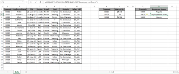
Let’s understand the working with an example as below (Figure 1: Employee Salary Data)
- A) Say you need to find the salary from Empcode.
- B) Say you need to find the Employee name from Empcode
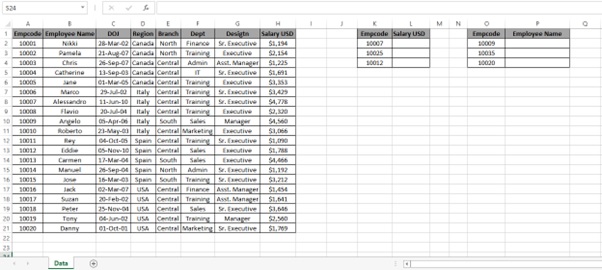
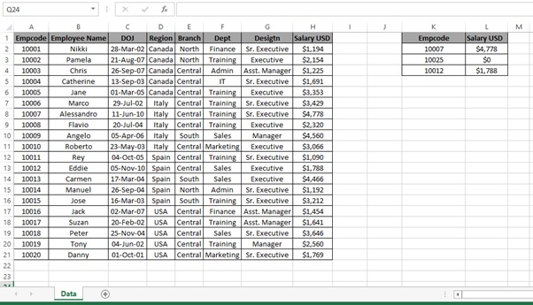
Figure 1: Employee Salary Data
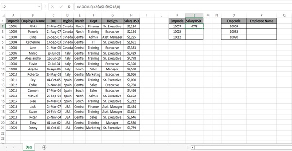
- A) To find the salary from Empcode.
Step 1: Type the below formula in cell L2.
=VLOOKUP(K2,$A$1:$H$21,8,0)
Step 2: Press Enter
We get the desired result.
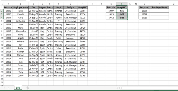
Step 3: Now drag the formula till cell L4.
You can see #N/A in Cell L3 (No value was found in the table for Empcode 10025)
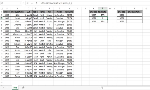
Step 4: Edit the formula as below
=IFERROR(VLOOKUP(K3,$A$1:$H$21,8,0),0)
Step 5: Press Enter
Step 6: Select L3 and select Ignore error from the options.
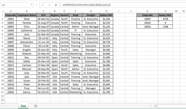
Step 7: We get the desired error result as 0.
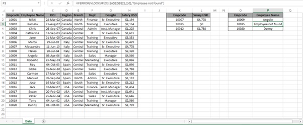
Step 8: After currency formatting.
- B) To find the Employee name from Empcode.
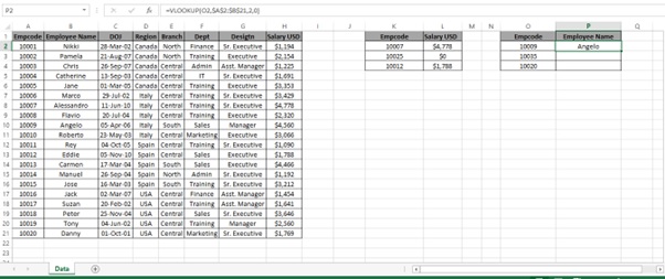
Step 1: Type the below formula in cell P2.
=VLOOKUP(O2,$A$2:$B$21,2,0)
Step 2: Press Enter
We get the desired result.
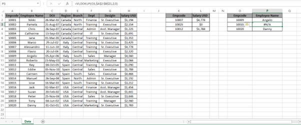
Step 3: Now drag the formula till cell P4.
You can see #N/A in Cell P3 (No value was found in the table for Empcode 10035)
Step 4: Edit the formula as below
=IFERROR(VLOOKUP(O3,$A$2:$B$21,2,0),”Employee not found”)
Step 5: Press Enter
Step 6: Select P3 and select Ignore error from the options.
Step 7: We get the desired error result.
Note: Instead of correcting the #N/A error after the error result we can Nest VLOOKUP() function inside the IFERROR() function first. In the above example we have shown the difference with and without IFERROR() function for your understanding.
Understanding how the formula works with the help of Evaluate Formula (Example 1)
Step 1: Select the cell (L3 in this case) that you want to evaluate. Only one cell can be evaluated at a time.
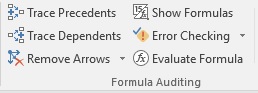
Step 2: On the Formulas tab click on Evaluate Formula in Formula Auditing group

Step 3: Evaluate Formula dialog box will appear.
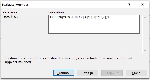
Step 4: Click Evaluate to examine the value of the underlined reference. The result of the evaluation is shown in italics.
If the underlined part of the formula is a reference to another formula, click Step In to display the other formula in the Evaluation box. Click Step Out to go back to the previous cell and formula.
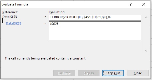
Step 5: After clicking on Step In button we get the lookup value.
Step 6: Click on Step Out
Step 7: VLOOKUP() function will be executed
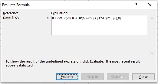
Step 8: #N/A is the result of VLOOKUP() function
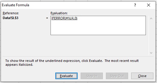
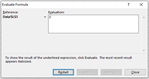
Step 9:. Result is 0
Understanding how the formula works with the help of Evaluate Formula (Example 2)
Step 1: Select the cell (P3 in this case) that you want to evaluate. Only one cell can be evaluated at a time.
Step 2: On the Formulas tab click on Evaluate Formula in Formula Auditing group
Step 3: Evaluate Formula dialog box will appear.
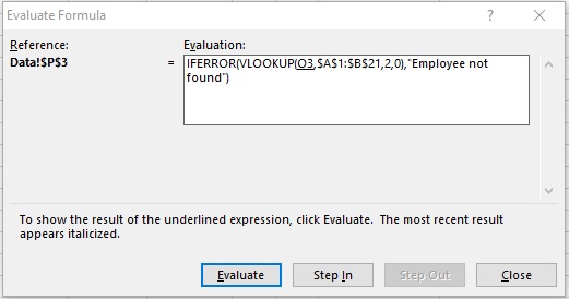
Step 4: Click Evaluate to examine the value of the underlined reference. The result of the evaluation is shown in italics.
If the underlined part of the formula is a reference to another formula, click Step In to display the other formula in the Evaluation box. Click Step Out to go back to the previous cell and formula.
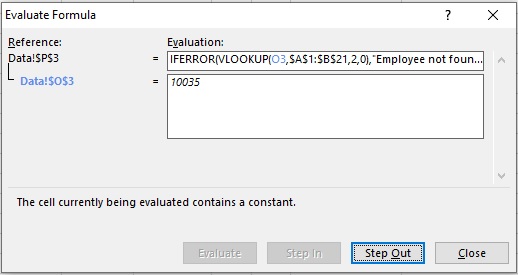
Step 5: After clicking on Step In button we get the lookup value.
Step 6: Click on Step Out
Step 7: VLOOKUP() function will be executed
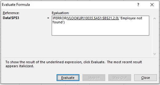
Step 8: #N/A is the result of VLOOKUP() function

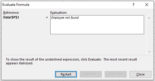
Step 9: Result is “Employee not found”.
Scope of Usage
- Can be used to customize the #N/A error
- Can be used with numeric values or non numeric values
- Can be used to provide a value of your own
- Can be used with IFERROR () function