Subject Line

Centralized View – Connect one Slicer to two pivot tables

Overview

Sometimes you may need to link one Slicer with two Pivot tables based on the same data source. Slicer is a powerful way to filter pivot table data. We can click on an item in a slicer to filter the data in the pivot table. Slicers provide buttons that you can click to filter tables or Pivot table.

Working

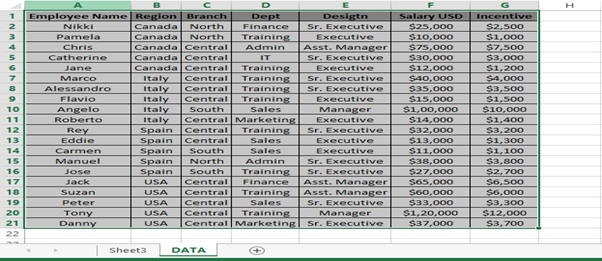
Let’s understand how with the help of an example (Figure 1: Employee Data)

You want to summarize designation wise salary and department wise salary from employee data with Region as filter.

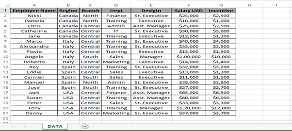
Figure 1: Employee Data

Step 1: Select the employee data from Column A to Column G from 1^st row till 21^st row.

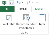
Step 2: Click on INSERT tab

Step 3: Click on PivotTable

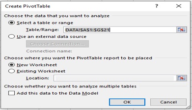
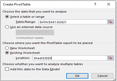
Step 4: Create PivotTable dialog box appears

Step 5: Click on OK

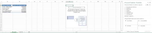
Step 6: Pivot Table sheet appears

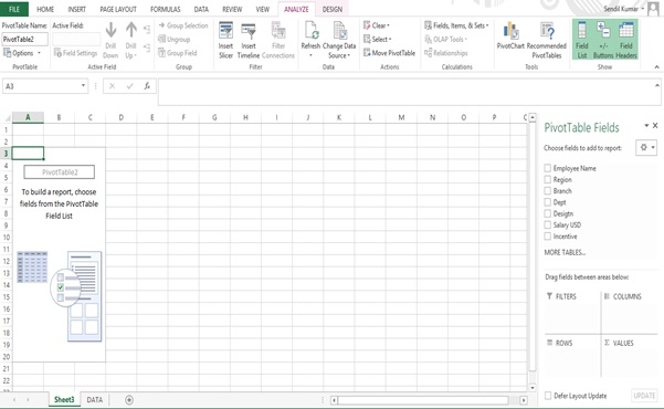
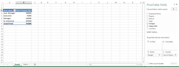
Step 7: Drag Design to ROWS area

Step 8: Drag Salary to VALUES area 

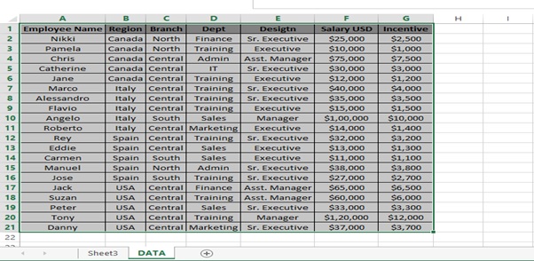
Step 9: Go to DATA Sheet

Step 10: Select the employee table from Column A to Column G from 1^st row till 21^st row.

Step 11: Click on INSERT tab

Step 12: Click on PivotTable

Step 13: Create PivotTable dialog box appears

Step 14: Select Existing Worksheet as we want to analyse both the Pivot Tables in the same sheet

Step 15: Change Location to Sheet3 and Cell I3

Step 16: Click on OK

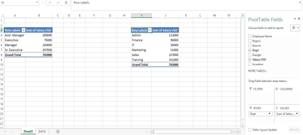
Step 17: Pivot Table sheet appears

Step 18: Drag Dept to ROWS area

Step 19: Drag Salary to VALUES area

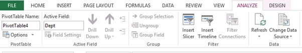
Step 20: Go to ANALYZE tab

Step 21: Click on Insert Slicer

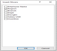
Step 22: Insert Slicers dialog box appears

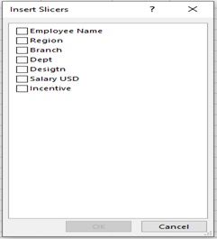
Step 23: Tick Region from the Insert Slicers option

Step 24: Click on OK

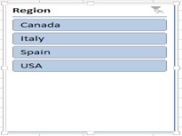
Step 25: Region slicer appears

Step 26: Now we have to connect slicer to both the PivotTables

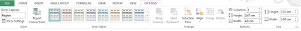
Step 27: Select the Region Slicer

Step 28: Go to OPTIONS tab

Step 29: Click on Report Connections

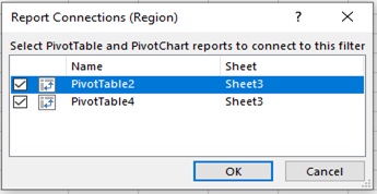
Step 30: Report Connections (Region) Dialog box appears

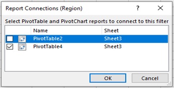
Step 31: Select PivotTable2 tick box

Step 32: Click on OK

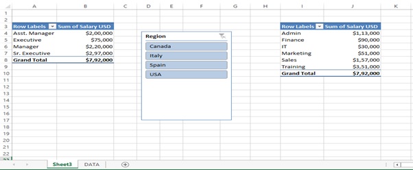
Step 33: Now Slicer is connected to both the PivotTables

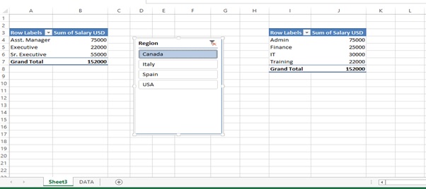
Step 34: Let’s check with Selecting Canada Region

Step 35: We get the correct result in both the Pivot Tables.

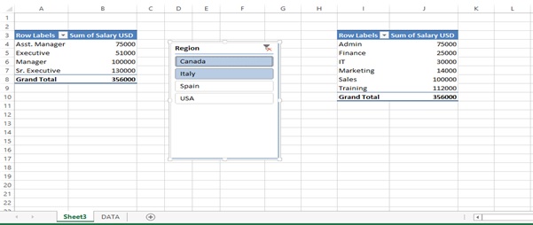
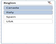
Step 36: Let’s select Canada & Italy region from the slicer by pressing Ctrl and selecting both the region

Step 37: We get the desired result in both the Pivot Tables.

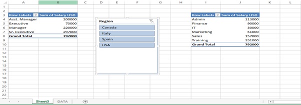
Step 38: After formatting the Salary in USD in both the Pivot Tables.

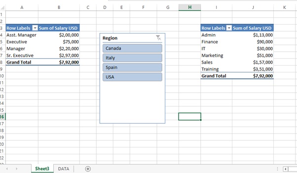
Step 39: Press Alt+C or Click on Clear Filter button provide in the Slicer box to clear the selection

Step 40: After clearing the slicer filter.

Scope of usage

• Can be used to filter data in a table or Pivot Table
• Can be used to connect one slicer to multiple Pivot Tables
• Can be used to analyze multiple Pivot Tables
• Can be used to create a central data view