Working

Let’s understand how we can link one slicer to 2 Pivot tables based on different data sources with the help of an example.

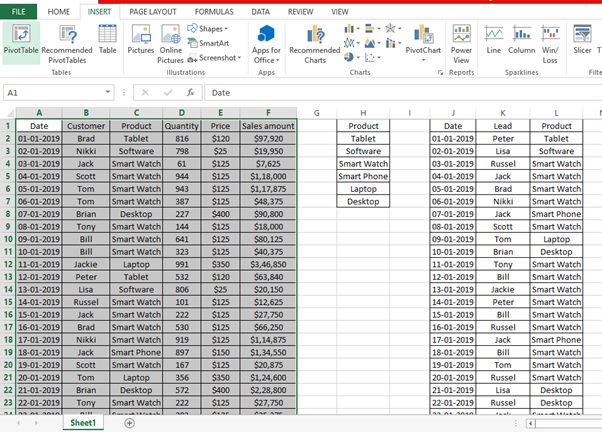
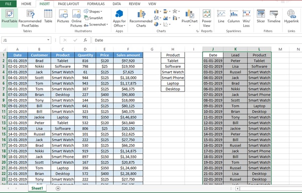
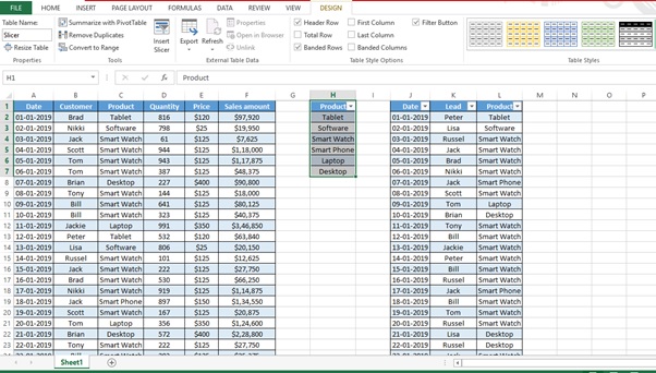
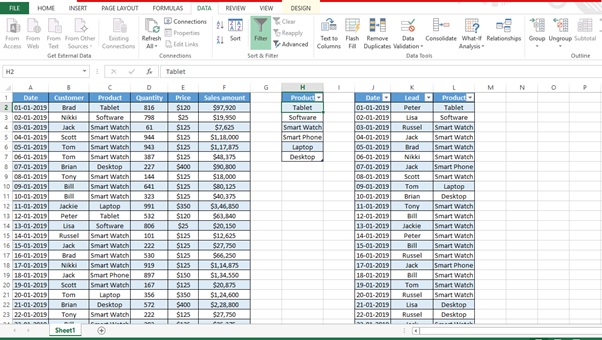
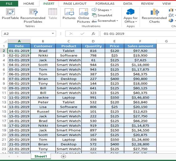
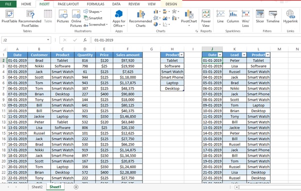
We have 2 Tables one is Sales table and other is the Lead Table.

We also have a Product table where we have only Product which are available in Sales table & Lead Table which will be used as a slicer.

We want to Summarize Customer wise Revenue from Sales table with number of Leads for the product from the Lead table (Figure 1: Two different sources)

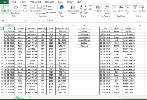
Figure 1: Two different sources

The steps are given as below

A.      CREATION OF SALES TABLE

Let’s create a Sales table with the help of the below steps.

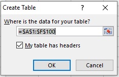
Step 1:  Select the data (A1:F100)

Step 2:  Click on INSERT tab

Step 3:  Click on Table in Tables group

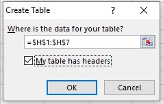
Step 4: Create table Dialog box appears

Step 5: Click on OK

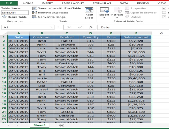
Step 6: Enter the table name as “Sales_tbl”

Step 7: Click on Enter

Step 8: Sales_tbltable is created 

 

B.      CREATION OF LEAD TABLE

Let’s create a Lead table with the help of the below steps.

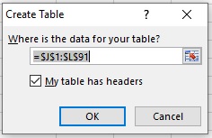
Step 1: Select the data (J1:L91)

Step 2: Click on INSERT tab

Step 3: Click on Table in Tables group

 

Step 4: Create table Dialog box appears

Step 5: Click on OK

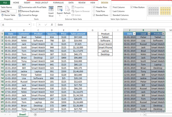
Step 6: Enter the table name as “Lead_Tbl”

Step 7: Click on Enter

Step 8: Lead_Tbltable is created

 

C.      CREATION OF SLICER TABLE

Let’s create a Slicer table with the help of the below steps.

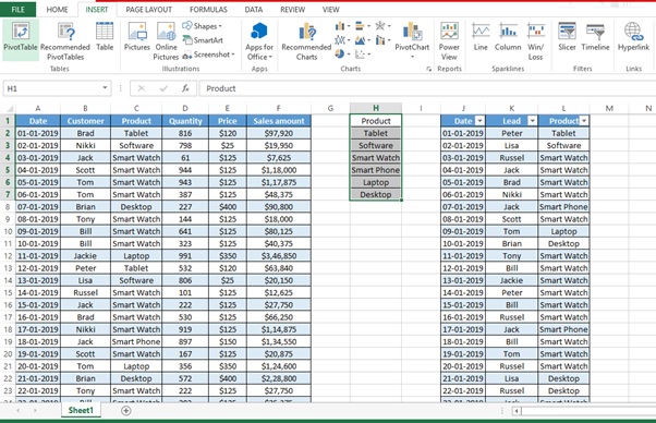
Step 1: Select the data (H1:H7)

Step 2: Click on INSERT tab

Step 3: Click on Table in Tables group

Step 4: Create table Dialog box appears

Step 5: Click on OK

Step 6: Enter the table name as “Slicer”

Step 7:  Click on Enter

Step 8:  Slicer table is created

D.      CREATION OF RELATIONSHIP

Let’s create relationship between Sales_tbl and Lead_Tbl

Step 1: Select the “Slicer” table

Step 2: Click on DATA tab

Step 3: Click on Relationship

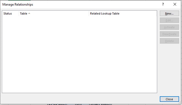
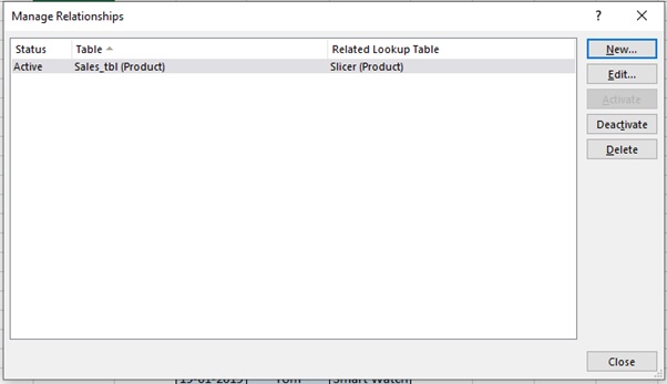
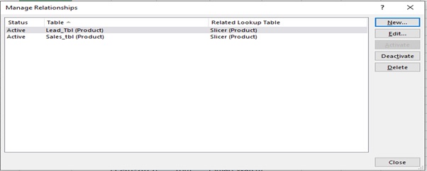
Step 4: Manage Relationships dialog box will appear

Step 5: Click on New

Step 6: Create Relationship dialog box will appear

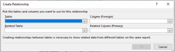
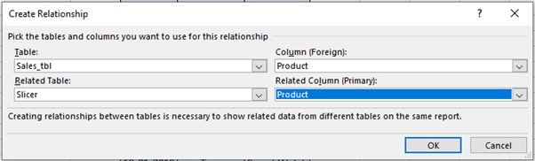
Step 7: Pick the Table and Column as per below image

We want to link Sales_tbl with Slicer table with Product as foreign and Primary key

Step 8: Click on OK

Step 9: Click on New

Step 10: Create Relationship dialog box will appear

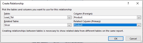
Step 11: Pick the Table and Column as per below image

We want to link Lead_Tbl with Slicer table with Product as foreign and Primary key

Step 12: Click on OK

Step 13: We have now created relationship with Slicer

E.       CREATION OF PIVOT AND LINKAGES

Let’s create 2 Pivot tables and link slicer to both the tables by following the below steps.

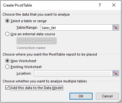
Step 1: Select any cell in the Sales_tbl table

Step 2: Click on INSERT tab

Step 3: Click on PivotTable

Step 4: Tick the “Add this data to the Data Model” checkbox

Step 5: Click on OK

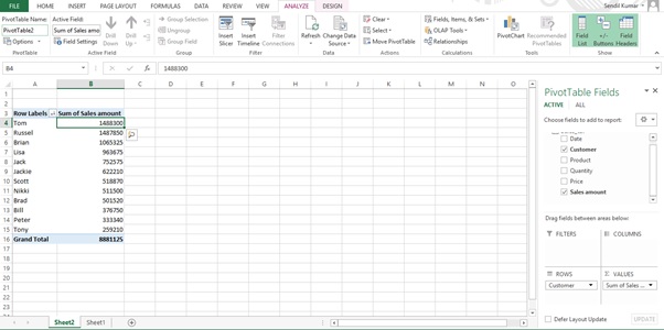
Step 6: Drag Customer to ROWS

Step 7: Drag Sales amount to VALUES

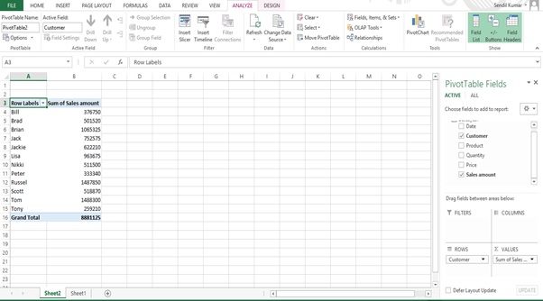
Step 8: Sort the Values(Sales amount) from Largest to Smallest

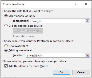
Step 9: Select any cell in the Lead_Tbltable

Step 10: Click on INSERT tab

Step 11: Click on PivotTable

Step 12: Select Existing Worksheet

Step 13: Go to Sheet 2 and select Cell H4

Step 14: Tick the “Add this data to the Data Model” checkbox

Step 15: Click on OK

 

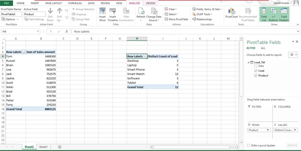
Step 15. Drag Product to ROWS

Step 16. Drag Lead to VALUES

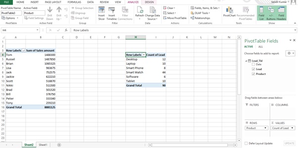
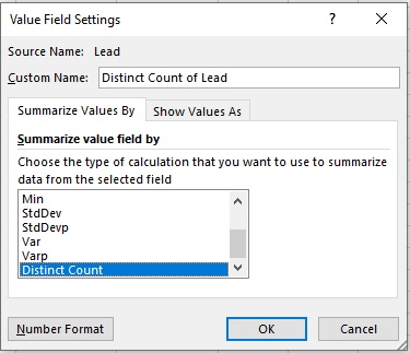
Step 16: Right click on Count of Lead

Step 17: Select Value Field Setting

Step 18: Select Distinct Count from Summarize values by tab

Step 19: Click on OK

Step 20: Sort the Sales amount by Largest to Smallest

Now we have to link the Slicer to both the tables.

Step 21: Select any cell from the Lead_Tbl Pivot table

Step 22: Click on Insert Slicer from Filter group in the ANALYZE tab

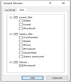
Step 23: Click on ALL tab

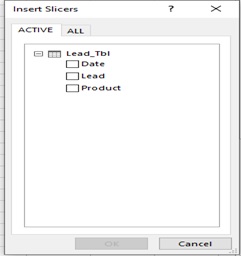
Step 24: Select Product from Slicer table

Step 25: Click on OK

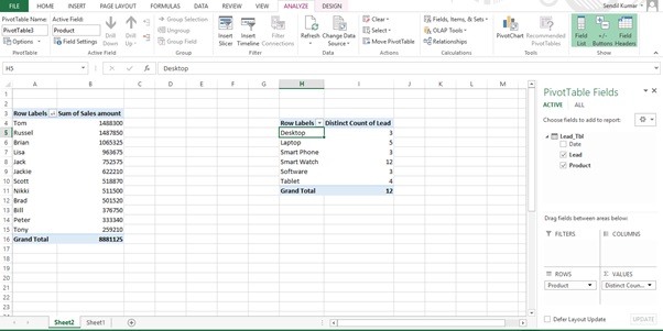
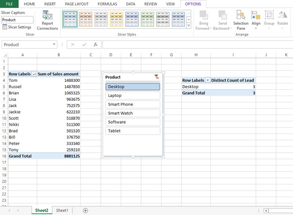
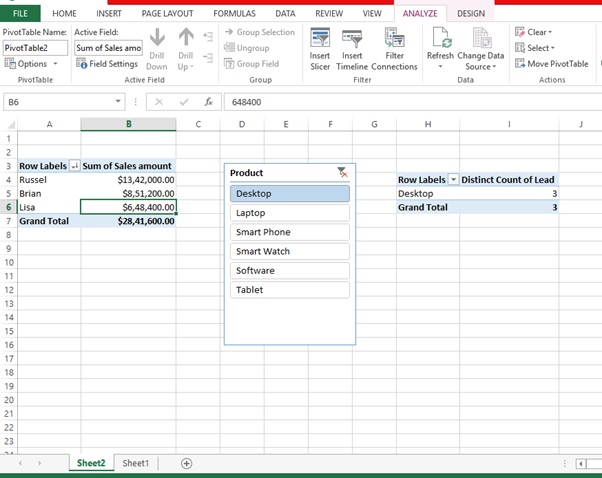
Step 26: Select Desktop from the slicer

Step 27: There is no change in the Sales_Tbl Pivot table

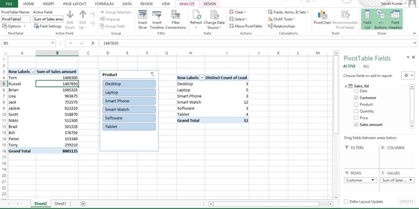
We have to connect the Sales_tbl Pivot table to the Slicer so that it also works with the Lead_Tbl Pivot table.

Step 28: Select any cell in Sales_tbl Pivot table

Step 29: Click on Filter Connections in the Filter group in the ANALYZE tab

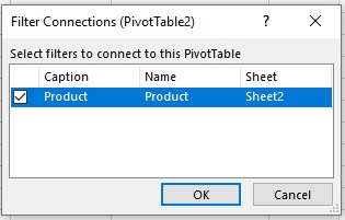
Step 30: Select the Product Checkbox

Step 31: Click on OK

Step 32: Change the Sales currency format to USD

Step 33: Select Desktop

Step 34: Now the filter is applied to both the tables using one slicer

 

Scope of usage

ü  Can be used to filter data in a table or a PivotTable

ü  Can be used to connect one slicer to multiple Pivot Tables

ü  Can be used to analyze from multiple tables

ü  Can be used to apply the slicers to multiple tables