Subject Line

There’s an in-built function to lookup values from the right side

Overview

Sometimes you may want to lookup value in a different way. There could be a table where you would want to use any column and then traverse from right to left to search according to the column. As you know the LOOKUP () function looks up values from left side and returns the value from the right hand side i.e. it works from left side of the table towards the right side of the table. What if you want to lookup value from the right side and return the value from the right side.

But there is a built in function specially designed for such case i.e. LOOKUP () Function.

Working

Let’s understand the working with the help of an example.

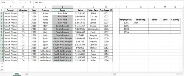
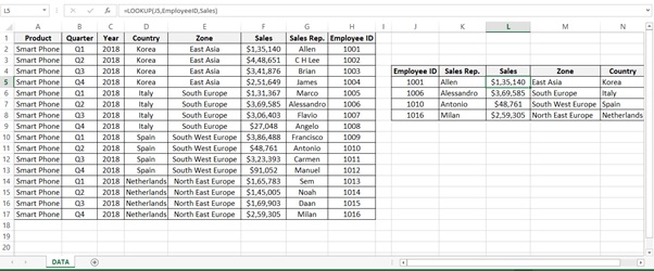
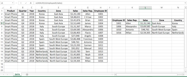
In the example used below Table 1: Sales of Smart Phones shows Sales of the Product (Smart Phone) by Year, Quarter, Country wise, Zone wise and Sales representative sales for their Zone.

Employee Id is the last column in the table (Column H)

The management wants a report in the format (Employee ID, Sales Rep, Sales, Zone and Country) for only a few Employee IDs. If you were to compare the report with the data the columns are in reverse order.

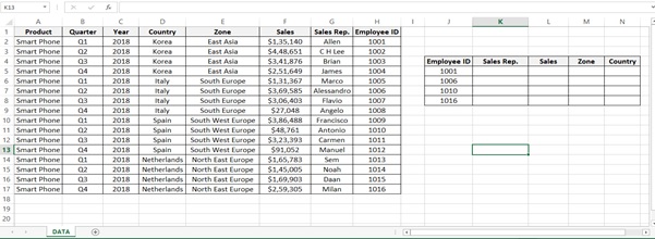
Table 1: Sales of Smart Phones

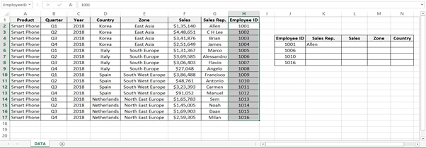
Step 1: Select the range of the employee ID H2 to H17.

Go to Name Box -> Type the NameEmployeeID in Name Box -> Click on Enter

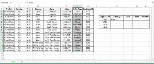
Step 2: Select the range of the Sales Rep. G2 to G17.

Go to Name Box -> Type the Name Sales_Rep in Name Box -> Click on Enter

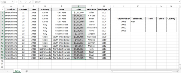
Step 3: Select the range of the Sales F2 to F17.

Go to Name Box -> Type the Name Sales in Name Bo -> Click on Enter

Step 4: Select the range of the Zone E2 to E17.

Go to Name Box -> Type the Name Zone in Name Bo -> Click on Enter

Step 5: Select the range of the Country D2 to D17.

Go to Name Box -> Type the Name Country in Name Bo -> Click on Enter

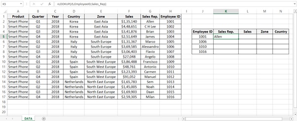
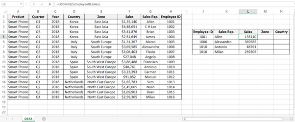
Step 6: To find the Sales Rep. name of Employee ID 1001 type the below formula.

= LOOKUP(J5,EmployeeID,Sales_Rep)

Syntax

= LOOKUP (lookup_value, lookup_vector, [result_vector])

Arguments

·         lookup_value – The value to search for.

·         lookup_vector – The one-row, or one-column range to search.

·         result_vector – [optional] The one-row, or one-column range of results.               

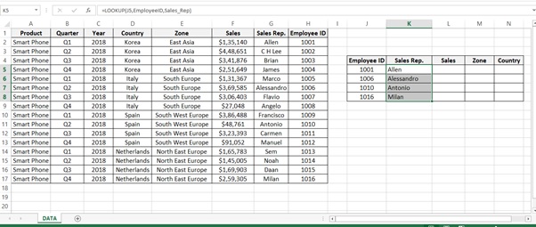
Step 7: Drag the formula for the all Employee ID. Select the cell and press Ctrl+D.

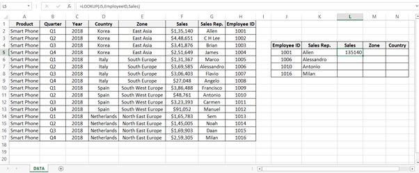
Step 8: To find the Sales of Employee ID 1001 type the below formula.

=LOOKUP(J5,EmployeeID,Sales)

Step 9: Drag the formula for the all Employee ID^. Select the cell and press Ctrl+D.

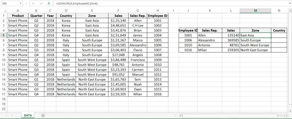
Step 10: To find the Zone of Employee ID 1001 type the below formula.

=LOOKUP(J5,EmployeeID,Zone)

Step 11: Drag the formula for the all Employee ID. Select the cell and press Ctrl+D.

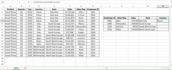
Step 12: To find the Country of Employee ID 1001 type the below formula.

=LOOKUP(J5,EmployeeID,Country)

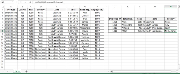
Step 13: Drag the formula for the all Employee ID’s. Select the cell and press Ctrl+D.

Step 14: Result after formatting the Sales amount

Understanding how the formula works with the help of Evaluate Formula

Step 1: Select the cell (K5 in this case) that you want to evaluate. Only one cell can be evaluated at a time.

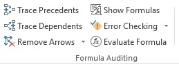
Step 2: On the Formulas tab click on Evaluate Formula in Formula Auditing group

Step 3: Evaluate Formula dialog box will appear

Click on Evaluate

It check the value of J5

Step 4: Value is 1001

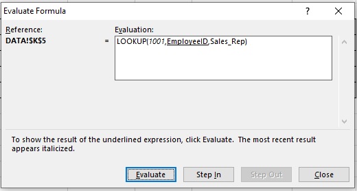
Step 5: Range of Employee ID range

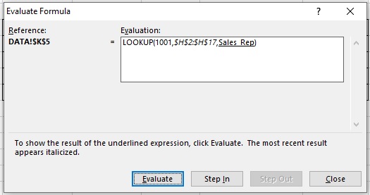
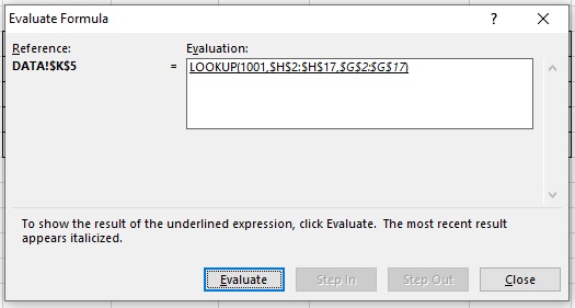
Step 6: Checks for Sales rep range.

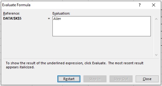
Step 7: Result is Allen

Scope of Usage

ü  Can be used as a built in function

ü  Can be used to perform a vertical lookup by searching for a value

ü  Can be used to lookup values from Right hand side of the table

ü  Can be used in situations when you need to reverse your search operation

ü  Can be used instead of INDEX () function and MATCH () function