Overview
Sometimes you may need to lookup values on matching patterns or search on part of the value eg: In case of Name you may want to search on the First Name or sometimes in case of any alphanumeric or numeric value you may want to search based on some particular way. You can replace the existence of characters by using wildcards to represent the number of characters. Basically your search pattern can be customized.
Let’s also understand the working of VLOOKUP () function
- The value you want to look up which is called the lookup value
- The range where the lookup value is located
Note: the lookup value should always be in the first column in the range for VLOOKUP to work correctly. For example, if your lookup value is in cell C2 then your range should start with C.
- The column number in the range that contains the return value. For example, if you specify B2:D11 as the range, you should count B as the first column, C as the second, and so on.
- Optionally, you can specify TRUE if you want an approximate match or FALSE if you want an exact match of the return value. If you don’t specify anything, the default value will always be TRUE or approximate match. You can also use 1 or 0
Working
The wildcard characters are
- Asterisk (*) – Finds any number of characters after a text.
- Question Mark (?) – Question mark is used to replace with a character.
Let’s understand the working with the help of examples
We have Sales data (Figure 1: Sales Data) for the year 2018 for the 5 Products
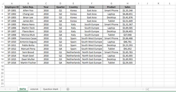
Figure 1: Sales Data
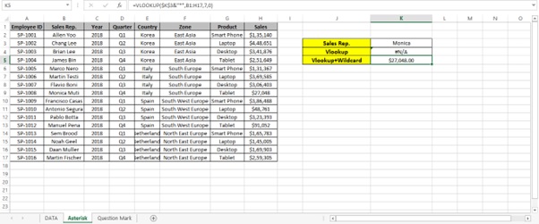
In the first example we have to find the Sales amount of Monica
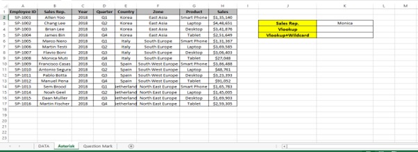
Step 1: Type the below VLOOKUP formula
=VLOOKUP(K3,B1:H17,7,0)
We get #N/A error as a result
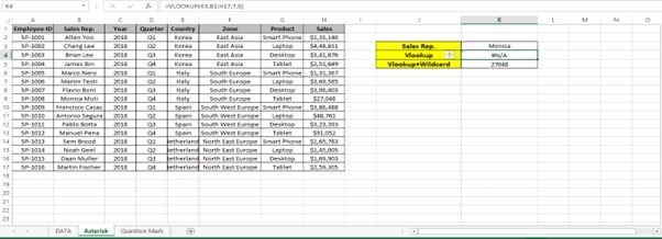
Step 2: Type the below VLOOKUP formula along with “*” wildcard character
=VLOOKUP($K$3&”*”,B1:H17,7,0)
Asterisk (*) Sign finds any number of characters after a text.
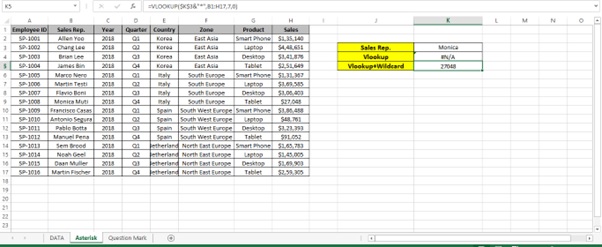
Step 3: After changing the currency format to $ English (United States) from the Symbol
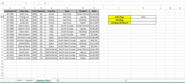
In the second example we have to find the Sales Rep. name of Employee ID 1011.

Step 1: Type the below VLOOKUP formula
=VLOOKUP(K3,$A$1:$B$17,2,0)
We get #N/A error as a result
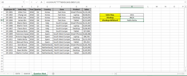
Step 2: Type the below VLOOKUP formula along with “????” wildcard character
=VLOOKUP(“???”&$K$3,$A$1:$B$17,2,0)
Question mark (?) sign is used to replace with a character
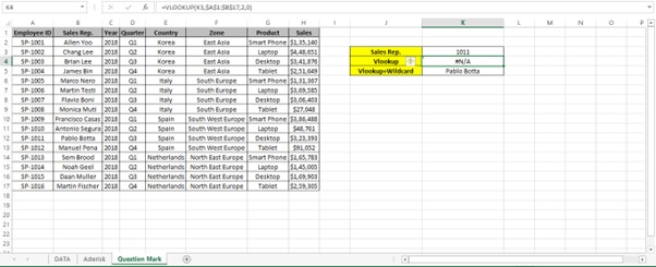
Step 3: Result
Understanding how the formula works with the help of Evaluate Formula (Example 1)
Step 1: Select the cell (K5 in this case) that you want to evaluate. Only one cell can be evaluated at a time.
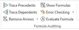
Step 2: On the Formulas tab click on Evaluate Formula in Formula Auditing group

Step 3: Evaluate Formula dialog box will appear.
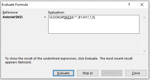
Step 4: Click Evaluate to examine the value of the underlined reference. The result of the evaluation is shown in italics.
If the underlined part of the formula is a reference to another formula, click Step In to display the other formula in the Evaluation box. Click Step Out to go back to the previous cell and formula.
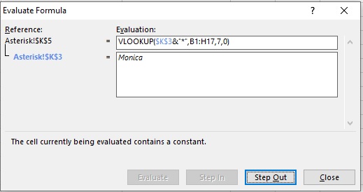
Step 5: Click on Evaluate
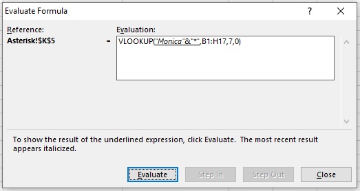
Step 6: Click on Evaluate

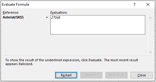
Step 7: Result
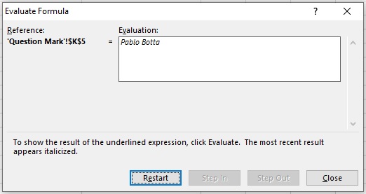
Understanding how the formula works with the help of Evaluate Formula (Example 2)
Step 1: Select the cell (K5 in this case) that you want to evaluate. Only one cell can be evaluated at a time.
Step 2: On the Formulas tab click on Evaluate Formula in Formula Auditing group
Step 3: Evaluate Formula dialog box will appear.
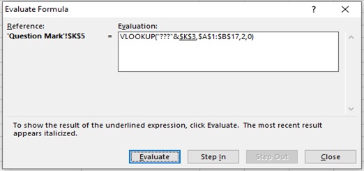
Step 4: Click Evaluate to examine the value of the underlined reference. The result of the evaluation is shown in italics.
If the underlined part of the formula is a reference to another formula, click Step In to display the other formula in the Evaluation box. Click Step Out to go back to the previous cell and formula.
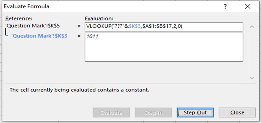
Step 5: Click on Evaluate

Step 6: Click on Evaluate
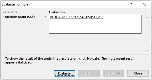
Step 7: Result
Scope of usage
- Can be used to customize your search patterns
- Can be used to lookup for a value using a partial match
- Can be used to lookup a value when there isn’t an exact match
- Can be used to replace a single or more characters while searching