Syntax
=INDEX(data,MATCH(val,rows,0),MATCH(val,columns,0))
Let’s understand both the function
INDEX function returns a value in a table based on the intersection of a row and column position within that table.
Syntax
=INDEX (array, row_num, [col_num], [area_num])
Arguments
· array – A range of cells, or an array constant.
· row_num – The row position in the reference or array.
· col_num – [optional] The column position in the reference or array.
· area_num – [optional] The range in reference that should be used.
Match option is used to locate the position of a lookup value in a row, column, or table.
Syntax
=MATCH (lookup_value, lookup_array, [match_type])
Arguments
· lookup_value – The value to match in lookup_array.
· lookup_array – A range of cells or an array reference.
· match_type – [optional] 1 = exact or next smallest (default), 0 = exact match, -1 = exact or next largest.
Working
Let’s understand the working with the help of an example.
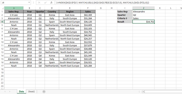
We have a report (Figure 1: Sales Report) for the year 2018.
We have to find the result based on the Sales Rep., Quarter and Criteria 3 (Country/Region/Sales) selection.
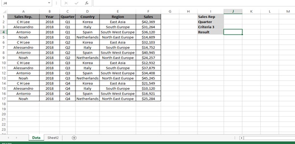
Figure 1: Sales Report
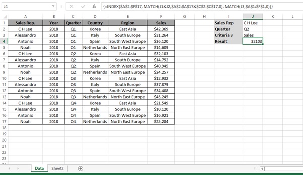
Step 1: Type the below formula
=INDEX($A$2:$F$17, MATCH(J1&J2,$A$2:$A$17&$C$2:$C$17,0), MATCH(J3,$A$1:$F$1,0))
What is Array Formula
An array formula is a formula that can perform multiple calculations on one or more items in an array.
Since this is an array formula, use it with Control + Shift + Enter, instead of just Enter.
{=INDEX($A$2:$F$17, MATCH(J1&J2,$A$2:$A$17&$C$2:$C$17,0), MATCH(J3,$A$1:$F$1,0))}
We get the desired result
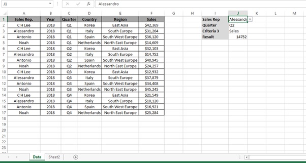
Step 2: Change the criteria from the drop down list to get the desired result
Understanding how the formula works with the help of Evaluate Formula
Step 1: Select the cell (J4 in this case) that you want to evaluate. Only one cell can be evaluated at a time.
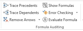
Step 2: On the Formulas tab click on Evaluate Formula in Formula Auditing group
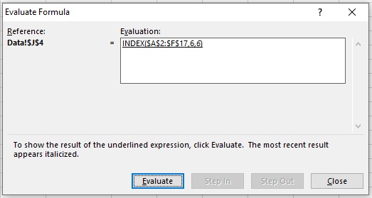
Step 3: Evaluate Formula dialog box will appear.
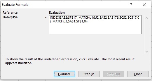
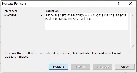
Step 4: Click Evaluate to examine the value of the underlined reference. The result of the evaluation is shown in italics.
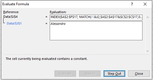
If the underlined part of the formula is a reference to another formula, click Step In to display the other formula in the Evaluation box. Click Step Out to go back to the previous cell and formula.
Step 5: Click on Evaluate
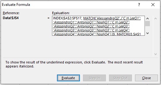
Step 6: Click on Evaluate
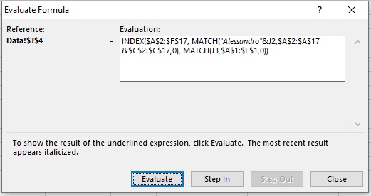
Step 7: Click on Evaluate
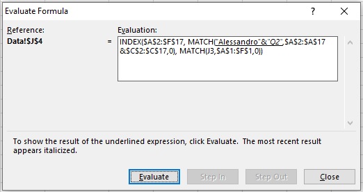
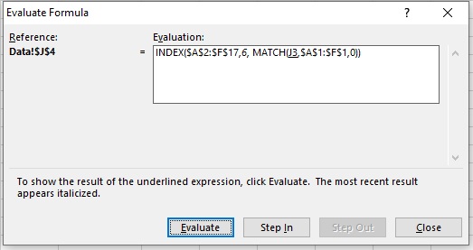
Step 8: Click on Evaluate
Step 9: Click on Evaluate
Step 10: Click on Evaluate
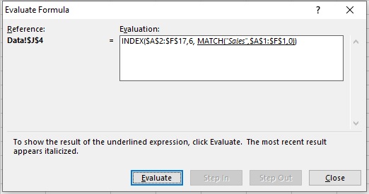
Step 11: Click on Evaluate
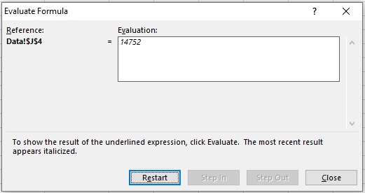
Step 12: Result
Step 13: Change the Sales Rep./Quarter/Criteria 3 to get the desired results
Scope of usage
ü Can be used with drop down lists
ü Can be used to build drop down lists
ü Can be used to retrieve values based on a combination
ü Can be used to VLOOKP () on two or more criteria columns
ü Can be used with INDEX () and MATCH () function