Syntax

=INDEX(data,MATCH(val,rows,0),MATCH(val,columns,0))

Let’s understand both the function

INDEX function returns a value in a table based on the intersection of a row and column position within that table.

Syntax

=INDEX (array, row_num, [col_num], [area_num])

Arguments

·         array – A range of cells, or an array constant.

·         row_num – The row position in the reference or array.

·         col_num – [optional] The column position in the reference or array.

·         area_num – [optional] The range in reference that should be used.

Match option is used to locate the position of a lookup value in a row, column, or table.

Syntax

=MATCH (lookup_value, lookup_array, [match_type])

Arguments

·         lookup_value – The value to match in lookup_array.

·         lookup_array – A range of cells or an array reference.

·         match_type – [optional] 1 = exact or next smallest (default), 0 = exact match, -1 = exact or next largest.

Working

Let’s understand the working with the help of an example.

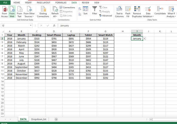
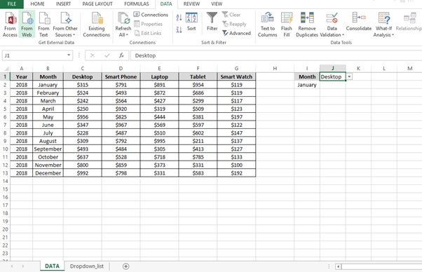
We have a report (Figure 1: Sales Report) for 5 Products for the year 2018.

In the below table we want to extract Sales amount of the Product based on Month and Product which will be provided in the drop down list.

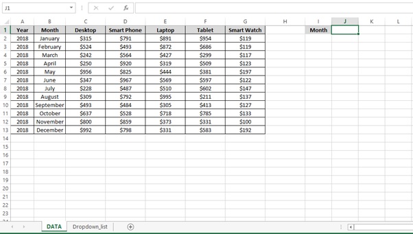
Figure 1: Sales Report

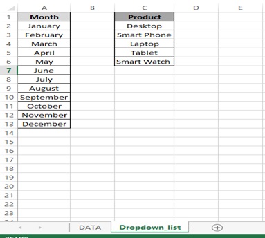
Step 1: Go to Dropdown list sheet and check the Month and Product list which will be used as Row and Column in the formula.

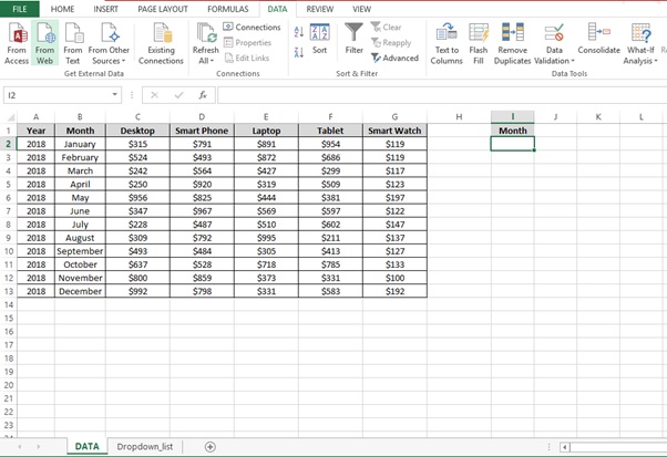
Step 2: Click on Cell I2

Step 3:  Go to DATA Tab

Step 4:  Click on Data Validation option in the Data Tools group

Step 5: Data Validation box will appear

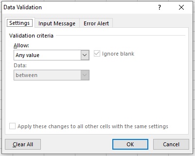
Step 6: Select List from Allow Option

Step 7: Click on Source range

Step 8:  Go to Dropdown_list sheet and select the month (January to December)

Step 9:  Click on OK

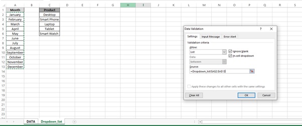
Step 10: We have now created Month dropdown in Cell I2

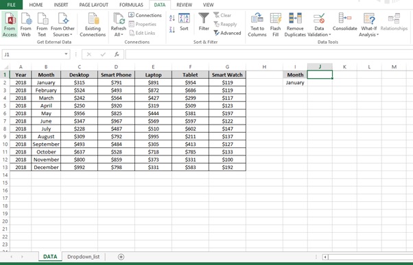
Step 11: Click on Cell J2

Step 12: Go to DATA Tab

Step 13: Click on Data Validation option in the Data Tools group

Step 14: Select List from Allow Option

Step 15: Click on Source range

Step 16: Go to Dropdown_list sheet and select the Product

Step 17: Click on OK

 

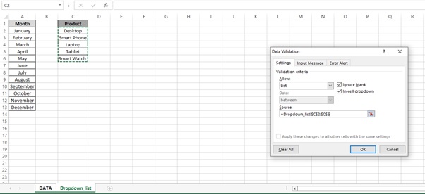
Step 18: We have now created Product dropdown in Cell J2

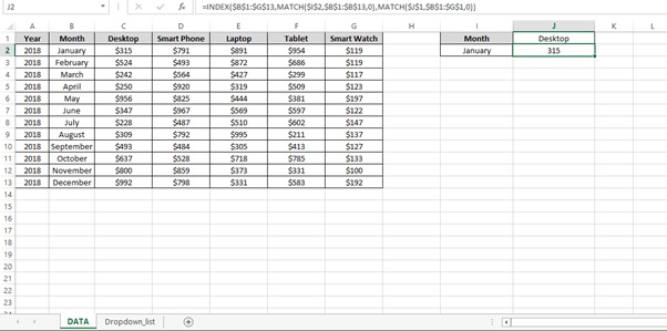
Step 19: Now enter the below formula.

=INDEX($B$1:$G$13,MATCH($I$2,$B$1:$B$13,0),MATCH($J$1,$B$1:$G$1,0))

 

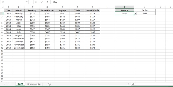
Step 20: Final Check

Select May Month and Tablet Product and see the result.

Understanding how the formula works with the help of Evaluate Formula

Step 1: Select the cell (J2 in this case) that you want to evaluate. Only one cell can be evaluated at a time.

Step 2: On the Formulas tab click on Evaluate Formula in Formula Auditing group

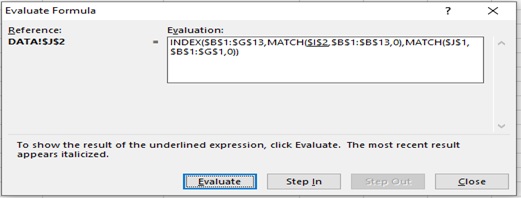
Step 3: Evaluate Formula dialog box will appear.

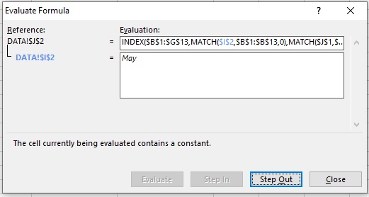
Step 4: Click Evaluate to examine the value of the underlined reference. The result of the evaluation is shown in italics.

If the underlined part of the formula is a reference to another formula, click Step In to display the other formula in the Evaluation box. Click Step Out to go back to the previous cell and formula.

Step 5: Click on Evaluate

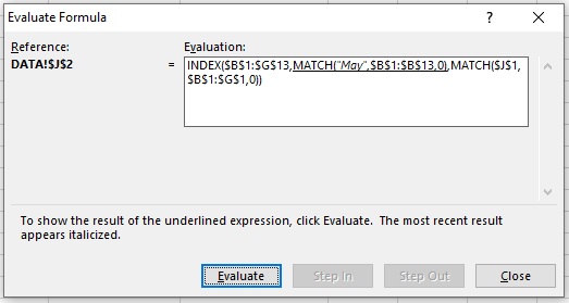
Step 6: Click on Evaluate

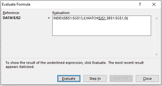
Step 7: Click on Evaluate

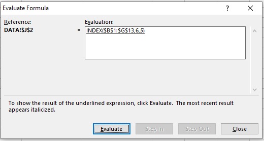
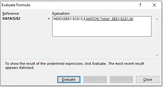
Step 8: Click on Evaluate

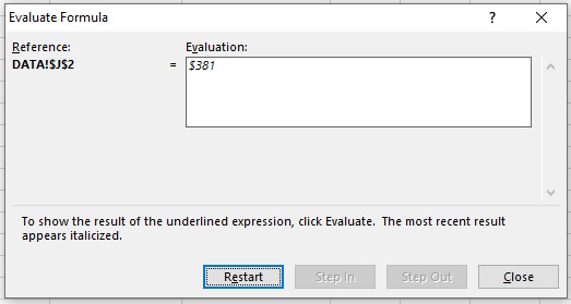
Step 9: Result

Scope of usage

ü  Can be used to build drop down list

ü  Can be used with drop down lists

ü  Can be used to perform two way lookup

ü  Can be used to retrieve values based on a combination of drop down selections

ü  Can be used with INDEX () and MATCH () function